Linear regression

Key takeaways

Linear regression is a supervised machine learning algorithm that models the relationship between a continuous dependent variable and one or more independent variables. It fits a linear equation to observed data.
The representation is a linear equation that combines input values (x) to predict the output value (y). It assigns a coefficient to each input, called Beta (B). One additional coefficient is the intercept or bias term.
Learning the model means estimating the coefficient values that best fit the training data. Common techniques include Ordinary Least Squares, Gradient Descent, and Regularization methods like Lasso and Ridge Regression.
Linear regression assumptions include linearity, independence, homoscedasticity, and normality of residuals. The data requires some preparation like removing outliers and noise.
Applications include predicting trends, forecasting, time series modeling, and determining causal relationships between variables. Limitations include being prone to overfitting and unable to model nonlinear relationships

Introduction

Linear regression is a statistical technique that models the relationship between a continuous dependent variable and one or more independent variables. It fits a linear equation to observed data using the method of least squares. Linear regression makes predictions by finding the line that minimizes the sum of the squares of the vertical distances between the observed responses in the dataset and the responses predicted by the linear approximation. Linear regression has been around for more than 200 years and has been widely used in economics, finance, biology, demography, and many other fields 1. In machine learning, linear regression is a supervised learning algorithm used for predictive analysis. This report provides an in-depth understanding of how the linear regression algorithm works, its key components, assumptions, applications, and limitations.

How Linear Regression works

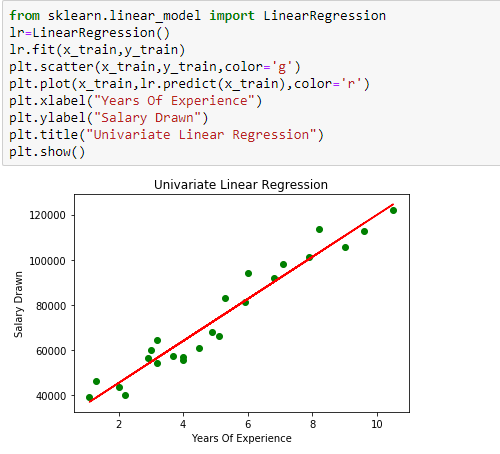
Linear regression fits a linear equation to model the relationship between a dependent variable y and one or more independent variables X . The linear equation assigns a coefficient to each input variable, called Beta (β). An additional intercept coefficient (β0) provides the line an additional degree of freedom. The representation of a simple linear regression with one input variable is:

 y = β0 + β1X

For multiple input variables, the representation is:

y = β0 + β1X1 + β2X2 + ... + βpXp

The coefficients (β) are estimated to minimize the sum of squared residuals between predicted and actual values of y. Predictions can then be made by plugging in values of the independent variables into the linear equation.

Key Components

The key components of a linear regression model are:

Dependent variable (y) : The continuous target variable that the model predicts. Also called the response variable.
Independent variables (X): The input variables used to predict the dependent variable. Also called explanatory or predictor variables
Coefficients (B): The coefficients assigned to each independent variable that quantify the relationship with the dependent variable.
Intercept (B0): The intercept coefficient that defines where the regression line intercepts the y-axis.
Residuals: The differences between actual and predicted values of the dependent variable. The model tries to minimize the sum of squared residuals.

Learning Algorithms

Some common algorithms used to learn the coefficients from data include:

Ordinary Least Squares: Finds coefficients that minimize the sum of squared residuals.
Gradient Descent: Iteratively updates coefficients to reduce cost and find optimal values. Requires tuning a learning rate parameter.
Lasso Regression: Penalizes sum of absolute coefficients to reduce model complexity.
Ridge Regression: Penalizes sum of squared coefficients to reduce model complexity.

Assumptions

Linear regression relies on several assumptions about the data:

Linear relationship: The relationship between dependent and independent variables is linear.
Independence: The residuals should not be correlated.
Homoscedasticity: The residuals should have constant variance at each level of the independent variables.
Normality: The residuals should be normally distributed, with mean 0.
No multicollinearity: The independent variables should not be highly correlated.

Applications

Some applications of linear regression include:

Predicting trends and future values
Time series modeling and forecasting
Determining causal relationships between variables
Estimating the effect of changing one variable on another variable

Limitations

Some limitations of linear regression include:

Prone to overfitting with many input variables
Unable to model nonlinear relationships
Sensitive to outliers that skew the regression line
Requires meeting assumptions about the data
Does not work well with categorical variables

Conclusion

Linear regression is a fundamental supervised learning technique used for predictive analysis. It models the linear relationship between a dependent variable and one or more independent variables. Key aspects include the model representation, learning algorithms, assumptions, applications, and limitations. With an understanding of how linear regression works, it can be effectively applied for making predictions and gaining insights from data in many domains.

References

Neter, J., Kutner, M. H., Nachtsheim, C. J., & Wasserman, W. (1996). Applied linear statistical models. Irwin.
How Linear regression algorithm works—ArcGIS Pro | Documentation. (2022).

here